Linear programming – problem formulation, simplex method and graphical solution, sensitivity analysis

Linear programming is a mathematical procedure to find out best solutions to problems that can be stated using linear equations and inequalities. If a real-world problem can be represented precisely by the mathematical equations of a linear program, the method will find the best solution to the problem. Linear programming is a comparatively complex technique. Linear programming can be explained as "A mathematical method to allocate scarce resources to competing activities in an optimal manner when the problem can be expressed using a linear objective function and linear inequality constraints." Linear programming uses linear algebraic relationships to signify a firm's decisions, given a business objective, and resource constraints.

It has been observed that Management decisions in many organizations involve to make appropriate use of resources such as machinery, labour, money, time, warehouse space, and raw materials, in order to produce products like computers, automobiles, or clothing or offer services such as package delivery, health services, or investment decisions. To solve problems of resource allocation, company adopt the technique of mathematical programming. Linear programming is the most common category of mathematical programming. Linear programming seeks to maximize or minimize a linear objective function subject to a set of linear constraints and assumes all relevant input data and parameters that are known with certainty. Computers are important in the solution of linear programming problems (Sharma, 2006).

In simple form, A linear program include a set of variables, a linear objective function indicating the contribution of each variable to the desired outcome, and a set of linear constraints describing the limits on the values of the variables. Linear programs are problems

Maximize	CT X
Subject to	Ax  ≤  b
and	x ≥ 0

Where, 'x' signifies the vector of variables (to be determined), c and b are vectors of (known) coefficients, A is a (known) matrix of coefficients, and (\cdot)^\mathrm (T) is the matrix transpose. The expression to be maximized or minimized is called the objective function (cTx in this case). The inequalities Ax ≤ b and x ≥ 0 are the constraints which specify a convex polytope over which the objective function is to be optimized. In this context, two vectors are comparable when they have the same dimensions. If every entry in the first is less-than or equal-to the corresponding entry in the second then we can say the first vector is less-than or equal-to the second vector.

Linear programming consists for four basic components:

1. Decision variables represent quantities to be determined.
2. Objective function represents how the decision variables affect the cost or value to be optimized (minimized or maximized).
3. Constraints represent how the decision variables use resources, which are available in limited quantities.
4. Data quantifies the relationships represented in the objective function and the constraints

Model Formulation Steps:
Step 1: Clearly define the decision variables
Step 2: Construct the objective function
Step 3: Formulate the constraints

Formulatıng a linear programming problem:
A common linear programming application is product mix problem. Two or more products are usually produced using limited resources, such as personnel, machines, raw materials. Profit firm seeks to maximize is based on profit contribution per unit of each product (Sharma, 2006). Firm would like to determine how many units of each product it should produce in order to maximize overall profit given its limited resources.

Simplex Method

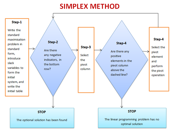
For linear programing problems involving more than two variables or problems with large number of constraints, it is useful to use solution methods that are adaptable to computers. Solving linear programing problems graphically is only practical when there are two decision variables. Furthermore, the graphical method becomes cumbersome when there are many constraints. Real-world LP problems typically have thousands of corner points. The appropriate technique in this situation is the simplex method, developed by George Dantzig in 1946. It provides us with a systematic way of examining the vertices of the feasible region to determine the optimal value of the objective function. The Simplex Method is matrix based method used for solving linear programming problems with any number of variables. The simplex algorithm can be used to solve linear programming problems that already are, or can be converted to, standard maximum-type problems.

It is established that the simplex method provides an iterative algorithm that methodically locates possible corner points that will improve the objective function value until the best solution is reached. Regardless of the number of decision variables and constraints, the simplex algorithm applies the key characteristic of any linear programing problem.

The general procedure of simplex method is as follows:

1. General form of given Linear Programming Problems is transformed to its canonical form.
2. A basic feasible solution of the Linear Programming Problems is found from the canonical form (there should exist at least one).
3. This initial solution is moved to an adjacent basic feasible solution which is closest to the optimal solution among all other adjacent basic feasible solutions.
4. The procedure is repeated until the optimum solution is achieved.

Simplex methods for standard maximization problems

Graphical solution:

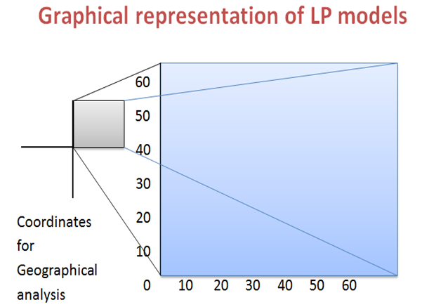
Graphical solution is limited to linear programming models containing any two decision variables. Graphical methods provide visualization of how a solution for a linear programming problem is obtained. Researcher can use graphical methods to solve linear optimization problems involving two variables. When there are two variables in the problem, they can refer to them as x1 and x2, and can do most of the analysis on a two-dimensional graph. Although the graphical approach does not generalize to a large number of variables, the basic concepts of linear programming can all be demonstrated in the two-variable context (Sharma, 2006).

Main advantage of the graphical approach is its visual nature. Graphical methods provide us with a picture to go with the algebra of linear programming, and the picture can anchor our understanding of basic definitions and possibilities. Therefore the graphical approach provides useful background for working with linear programming concepts.

Sensitivity Analysis

Sensitivity analysis allows researcher to determine how "sensitive" the optimal solution is to changes in data values. When an optimal solution is reached, management want to know how the optimal values would react to a change in the initial formulation of the linear programming problem, but it is not practical to redraft the entire problem for each possible change. Luckily, the information can be obtained directly through an analytical approach called sensitivity analysis. Sensitivity analysis fundamentally looks at the question of "what if" a variable is different from that originally estimated. The extensive use of computers has made sensitivity analysis a common extension of linear programming. Most linear programming computer packages include the results of sensitivity analysis as a part of the normal printout.

Application of linear programming: Linear programming can be used in various areas of study. It is used in business and economics, but can also be applied for engineering problems. Industries that practise linear programming models include transportation, energy, telecommunications, and manufacturing. It has proved useful in modelling diverse types of problems in planning, routing, scheduling, assignment, and design (Sharma, 2006). In spite of numerous advantages, linear programming has certain limitations:

1. To identify an objective function in mathematical form is not simple task.
2. Even if objective function is determined, it is problematic to determine social, institutional, financial and other constraints.
3. It is also possible that the objective function and constraints may not be directly specified by linear in equality equations.
4. To determine the relevant values of the co-efficient of constraints involved in LP is a main problem.
5. The assumptions of LP are also unrealistic. It assumes that factory proportion remains constant. In addition for it, the relationship between input and output, production and cost, and production and total revenue are assumed to be linear.

To summarize, Linear Programming is an important generalization of Linear Algebra. Linear Programming is used to successfully model numerous real world situations. The technique is prevailing and found especially useful because of its application to many different types of real business problems in areas such as finance, production, sales and distribution, personnel, marketing and many more areas of management. The linear programming model include linear objectives and linear constraints, which means that the variables in a model have a proportionate relationship.