Time Series and Forecasting

A time series is an assemblage of data recorded over a period of time whether it is weekly, monthly, quarterly, or yearly. A time series can be used by management to make existing decisions and plans based on long-term forecasting. Long-range forecasts are vital as they allow sufficient time for the procurement, manufacturing, sales, finance, and other departments of a company to devise plans for possible new plants, financing, development of new products, and new procedures of collecting. In sales, forecasting the level of, whether both short-term and long-term, is practically dictated by the very nature of business organizations. Factors like competition for the consumer's budget, pressure to generate a profit for the stockholders, a wish to obtain a larger share of the market, and the desires of managers are motivating forces in business. Therefore, a forecast (a statement of the goals of management) is needed to have the raw materials, production facilities, and staff available to meet the projected demand.

Component of time series: There are four components to a time series: the trend, the cyclical variation, the seasonal variation, and the irregular variation.

Trend component: The trend is the long term pattern of a time series. A trend can be positive or negative depending on whether the time series exhibits an increasing long term pattern or a decreasing long term pattern. If a time series does not represent an increasing or decreasing pattern then the series is static in the mean.

Cyclical Variation: The second component of a time series is cyclical variation. A typical business cycle comprises of a period of success followed by periods of recession, depression, and then recovery with no fixed duration of the cycle. There are substantial fluctuations describing over more than one year in time above and below the secular trend.

Seasonal Variation: The third constituent of a time series is the seasonal component. Many sales, production, and other series vary with the seasons. The unit of time reported is either quarterly or monthly.

Irregular Variation: The fourth elements of time series is irregular variations. Many analysts subdivide the irregular variation into episodic and residual variations. Episodic fluctuations are unpredictable, but they can be identified. The primary impact on the economy of a major strike or a war can be identified, but a strike or war cannot be predicted. After the episodic fluctuations have been removed, the remaining variation is called the residual variation. The residual fluctuations, also known as chance fluctuations, are unpredictable, and they cannot be recognised.

There are two major techniques of time series that include Open-model time series (OMTS) and fixed model time series (FMTS) techniques.

Fixed-model time series (FMTS) techniques are simple and economical to use and require little data storage. Many of the techniques also amend very quickly to changes in sales conditions and, therefore, are appropriate for short-term forecasting. Fixed-model time series techniques have fixed equations that are based upon a priori assumptions that certain patterns do or do not exist in the data.

The simplest form of an average as a forecast can be represented by the following formula:

where: S = Sales
N = Number of Periods of Sales Data (t)
It can be established that forecast for next month (or any month in the future, for that matter) is the average of all sales that have occurred in the past. The benefit to the average as a forecast is that the average is designed to reduce any fluctuations. Thus, the average takes the noise (which time series techniques assume cannot be forecasted anyway) out of the forecast. However, the average also dampens out of the forecast any fluctuations, including such important fluctuations as trend and seasonality.

The average as a forecasting method has the additional disadvantage that it requires enormous amount of data storage. With the data storage capabilities of contemporary computers, this may not be too burdensome a disadvantage, but it does cause the average to be inactive to changes in level of demand. All FMTS techniques were developed to overcome some drawback of the average as a forecast.

Open-model time series: Open-model time series (OMTS) techniques investigate the time series to regulate which patterns exist and then build a unique model of that time series to project the patterns into the future and thus to forecast the time series. Open-model time series techniques undertake that the same mechanisms exist in any time series level, trend, seasonality, and noise but take a different approach to forecasting these components. OMTS techniques first analyse the components in the time series to understand which exist and what their nature is. From this information, a set of forecasting formulae unique to that time series is built.

Numerous types of Open-model time series exist that include decomposition analysis (Shiskin 1961a, 1961b), spectral analysis (Nelson, 1973), fourier analysis (Bloomfield, 1976), and auto-regressive moving average (ARMA) or Box-Jenkins analysis (Box and Jenkins, 1970). All of these Open-model time series techniques have common factor that they first try to scrutinize the time series to determine the components and, as a result, require a significant amount of history before any forecasts can be made. The analysis with Open-model time series is a difficult task and requires substantial input from the forecaster. Due to this, Open-model time series techniques are not extensively used in practice (Mentzer and Kahn, 1995).

Applications of time-series forecasting: Time series forecasting is applied in following areas:

1. Economic planning
2. Sales forecasting
3. Inventory (or stock) control
4. Production and capacity planning
5. The evaluation of alternative economic strategies
6. Budgeting
7. Financial risk management
8. Model evaluation

Forecasting is a vital activity in economics, commerce, marketing and various branches of science. It is the process of making predictions of the future based on past and present data and analysis of trends. A forecasting technique is for computing forecasts from present and past values. As such it may simply be an algorithmic rule and need not depend on an underlying probability model. It may arise from identifying a particular model for the given data and finding best forecasts conditional on that model. It has been established that many types of forecasting models that differ in complexity and amount of data & way they generate forecasts are rarely perfect. Forecasts are more accurate for grouped data than for individual items and forecast are more accurate for shorter than longer time periods.

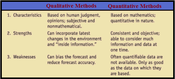
Forecasting methods are classified into two groups:
Qualitative methods are judgmental methods in which Forecasts generated subjectively by the forecaster. Quantitative methods are based on mathematical modelling in which Forecasts generated through mathematical modelling.

Univariate methods of forecasts denotes that forecasts depend only on present and past values of the single series being forecasted, possibly augmented by a function of time such as a linear trend.

Multivariate methods where forecasts of a given variable depend, at least partly, on values of one or more additional time series variables, called predictor or explanatory variables. Multivariate forecasts may depend on a multivariate model involving more than one equation if the variables are jointly dependent.

To summarize, a time-series is a collection of observations made successively through time. Forecasting is a technique for guessing future aspects of a business or the operation. It is a method for converting past data or experience into estimates of the future. This tool helps management in its attempts to cope with the ambiguity of the future.